helper_functions.py
A collection of (mostly) stand alone helper functions.
Miscellaneous functions
-
setDefaultArgs(func, **kwargs)[source]¶ Changes the default args in func to match kwargs.
This can be useful when dealing with deeply nested functions for which the default parameters cannot be set directly in the top-level function.
Raises: ValueError– if func does not have default arguments that match kwargs.Example
>>> def foo(bar="Hello world!"):
...     print bar
>>> setDefaultArgs(foo, bar="The world has changed!")
>>> foo()
The world has changed!
Numerical integration
-
rkqs(y, dydt, t, f, dt_try, epsfrac, epsabs, args=())[source]¶ Take a single 5th order Runge-Kutta step with error monitoring.
This function is adapted from Numerical Recipes in C.
The step size dynamically changes such that the error in y is smaller than the larger of epsfrac and epsabs. That way, if one wants to disregard the fractional error, set epsfrac to zero but keep epsabs non-zero.
Parameters: - dydt (y,) – The initial value and its derivative at the start of the step.
They should satisfy
dydt = f(y,t). dydt is included here for efficiency (in case the calling function already calculated it). - t (float) – The integration variable.
- f (callable) – The derivative function.
- dt_try (float) – An initial guess for the step size.
- epsabs (epsfrac,) – The maximual fractional and absolute errors. Should be either length 1 or the same size as y.
- args (tuple) – Optional arguments for f.
Returns: - Delta_y (array_like) – Change in y during this step.
- Delta_t (float) – Change in t during this step.
- dtnext (float) – Best guess for next step size.
Raises: IntegrationError– If the step size gets smaller than the floating point error.References
Based on algorithms described in [1].
[1] W. H. Press, et. al. “Numerical Recipes in C: The Art of Scientific Computing. Second Edition.” Cambridge, 1992. - dydt (y,) – The initial value and its derivative at the start of the step.
They should satisfy
Numerical derivatives
The derivij() functions accept arrays as input and return arrays as output.
In contrast, gradientFunction and :class:hessianFunction` accept
functions as input and return callable class instances (essentially functions)
as output. The returned functions can then be used to find derivatives.
-
deriv14(y, x)[source]¶ Calculates \(dy/dx\) to fourth-order in \(\Delta x\) using finite differences. The derivative is taken along the last dimension of y.
Both y and x should be numpy arrays. The derivatives are centered in the interior of the array, but not at the edges. The spacing in x does not need to be uniform.
-
deriv14_const_dx(y, dx=1.0)[source]¶ Calculates \(dy/dx\) to fourth-order in \(\Delta x\) using finite differences. The derivative is taken along the last dimension of y.
The output of this function should be identical to
deriv14()when the spacing in x is constant, but this will be faster.Parameters: - y (array_like) –
- dx (float, optional) –
-
deriv1n(y, x, n)[source]¶ Calculates \(dy/dx\) to nth-order in \(\Delta x\) using finite differences. The derivative is taken along the last dimension of y.
Both y and x should be numpy arrays. The derivatives are centered in the interior of the array, but not at the edges. The spacing in x does not need to be uniform.
-
deriv23(y, x)[source]¶ Calculates \(d^2y/dx^2\) to third-order in \(\Delta x\) using finite differences. The derivative is taken along the last dimension of y.
Both y and x should be numpy arrays. The derivatives are centered in the interior of the array, but not at the edges. The spacing in x does not need to be uniform. The accuracy increases to fourth-order if the spacing is uniform.
-
deriv23_const_dx(y, dx=1.0)[source]¶ Calculates \(d^2y/dx^2\) to third-order in \(\Delta x\) using finite differences. The derivative is taken along the last dimension of y.
The output of this function should be identical to
deriv23()when the spacing in x is constant, but this will be faster.Parameters: - y (array_like) –
- dx (float, optional) –
-
class
gradientFunction(f, eps, Ndim, order=4)[source]¶ Make a function which returns the gradient of some scalar function.
Parameters: - f (callable) – The first argument x should either be a single point with length
Ndim or an array (or matrix, etc.) of points with shape
(..., Ndim), where...is some arbitrary shape. The return shape should be the same as the input shape, but with the last axis stripped off (i.e., it should be a scalar function). Additional required or optional arguments are allowed. - eps (float or array_like) – The small change in x used to calculate the finite differences. Can either be a scalar or have length Ndim.
- Ndim (int) – Number of dimensions for each point.
- order (2 or 4) – Calculate the derivatives to either 2nd or 4th order in eps.
Example
>>> def f(X):
...     x,y = np.asarray(X).T
...     return (x*x + x*y +3.*y*y*y).T
>>> df = gradientFunction(f, eps=.01, Ndim=2, order=4)
>>> x = np.array([[0,0],[0,1],[1,0],[1,1]])
>>> print df(x)
    array([[ 0.,  0.], [ 1.,  9.], [ 2.,  1.], [ 3., 10.]])
-
__call__(x, *args, **kwargs)[source]¶ Calculate the gradient. Output shape is the same as the input shape.
-
__weakref__¶ list of weak references to the object (if defined)
- f (callable) – The first argument x should either be a single point with length
Ndim or an array (or matrix, etc.) of points with shape
-
class
hessianFunction(f, eps, Ndim, order=4)[source]¶ Make a function which returns the Hessian (second derivative) matrix of some scalar function.
Parameters: - f (callable) – The first argument x should either be a single point with length
Ndim or an array (or matrix, etc.) of points with shape
(..., Ndim), where...is some arbitrary shape. The return shape should be the same as the input shape, but with the last axis stripped off (i.e., it should be a scalar function). Additional required or optional arguments are allowed. - eps (float or array_like) – The small change in x used to calculate the finite differences. Can either be a scalar or have length Ndim.
- Ndim (int) – Number of dimensions for each point.
- order (2 or 4) – Calculate the derivatives to either 2nd or 4th order in eps.
-
__call__(x, *args, **kwargs)[source]¶ Calculate the gradient. Output shape is
input.shape + (Ndim,).
-
__weakref__¶ list of weak references to the object (if defined)
- f (callable) – The first argument x should either be a single point with length
Ndim or an array (or matrix, etc.) of points with shape
Two-point interpolation
-
makeInterpFuncs(y0, dy0, d2y0, y1, dy1, d2y1)[source]¶ Create interpolating functions between two points with a quintic polynomial.
If we’re given the first and second derivatives of a function at x=0 and x=1, we can make a 5th-order interpolation between the two.
-
class
cubicInterpFunction(y0, dy0, y1, dy1)[source]¶ Create an interpolating function between two points with a cubic polynomial.
Like
makeInterpFuncs(), but only uses the first derivatives.
Spline interpolation
-
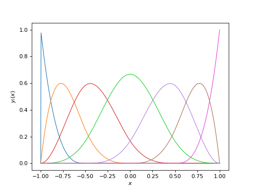
Nbspl(t, x, k=3)[source]¶ Calculate the B-spline basis functions for the knots t evaluated at the points x.
Parameters: - t (array_like) – An array of knots which define the basis functions.
- x (array_like) – The different values at which to calculate the functions.
- k (int, optional) – The order of the spline. Must satisfy
k <= len(t)-2.
Returns: array_like – Has shape
(len(x), len(t)-k-1).Notes
This is fairly speedy, although it does spend a fair amount of time calculating things that will end up being zero. On a 2.5Ghz machine, it takes a few milliseconds to calculate when
len(x) == 500; len(t) == 20; k == 3.For more info on basis splines, see e.g. http://en.wikipedia.org/wiki/B-spline.
Example
from cosmoTransitions.helper_functions import Nbspl
t = [-1,-1,-1,-1, -.5, 0, .5, 1, 1, 1, 1]
x = np.linspace(-1,1,500)
y = Nbspl(t,x, k=3)
plt.plot(x, y)
plt.xlabel(r"$x$")
plt.ylabel(r"$y_i(x)$")
plt.show()
(Source code, png, hires.png, pdf)